Estimate cell density in bands from a tissue boundary.

Given a cell seg table and an image containing masks for two tissue classes, estimate the density of cells of each specified phenotype in bands from the boundary between the two tissue classes.

density_bands(
  cell_seg_path,
  phenotypes,
  positive,
  negative,
  width = 25,
  map_path = NULL,
  component_path = NULL
)

Arguments

cell_seg_path

Path to a cell segmentation data file.

phenotypes

Optional named list of phenotypes to process. names(phenotypes) are the names of the resulting phenotypes. The values are in any format accepted by select_rows. If omitted, will use all phenotypes in the cell seg data.

positive

Name of the tissue category used as positive distance, e.g. "stroma".

negative

Name of the tissue category used as negative distance, e.g. "tumor".

width

Width of the bands, in microns

map_path

Path to the segmentation map file. If NULL, look for the map in the same directory as cell_seg_path.

component_path

Path to the component_data file corresponding to cell_seg_path; if omitted, look for the component data file in the same directory as cell_seg_path.

Value

Returns a list with three items:

densities

A tibble with five columns (see below).

cells

Cell seg data with phenotypes updated per the phenotypes parameter and an additional distance column.

distance

The distance map, a pixel image (im.object).

The densities item contains five columns:

phenotype

The supplied phenotypes.

midpoint

The midpoint of the distance band.

count

The number of cells of the phenotype found within the band.

area

The area of the band, in square microns.

density

The density of cells of the phenotype in the band, in cells per square micron.

Details

density_bands uses a counting approach similar to a histogram. First the image is divided into bands based on distance from the specified boundary. Next, the number of cells of each phenotype within each distance band is counted and the area of each band is estimated. The density estimates are the ratios of the cell counts to the area estimates.

Density estimates are in cells per square micron; multiply by 1,000,000 for cells per square millimeter.

The returned value includes the cell counts and area of each band, making it straightforward to aggregate across multiple fields from a single sample. The aggregate density is computed by summing the cell counts and areas across all fields from a sample, then dividing to compute density.

See also

Other density estimation: density_at_distance()

Examples

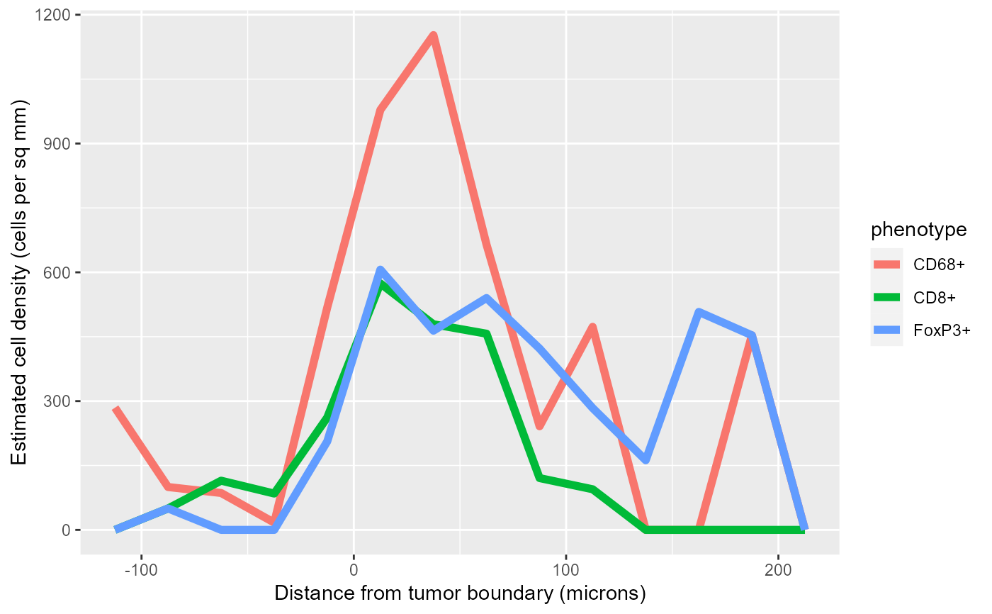
# Compute density for the sample data
values <- density_bands(sample_cell_seg_path(),
  list("CD8+", "CD68+", "FoxP3+"),
  positive="Stroma", negative="Tumor")

# Plot the densities in a single plot
library(ggplot2)
ggplot(values$densities, aes(midpoint, density*1000000, color=phenotype)) +
  geom_line(size=2) +
  labs(x='Distance from tumor boundary (microns)',
       y='Estimated cell density (cells per sq mm)')