Estimate cell density at distance from a tissue boundary.

Given a cell seg table and an image containing masks for two tissue classes, estimate the dependence of the density of cells of each phenotype on the distance from the boundary between the two tissue classes.

density_at_distance(
  cell_seg_path,
  phenotypes,
  positive,
  negative,
  mask = FALSE,
  pixels_per_micron = getOption("phenoptr.pixels.per.micron"),
  ...
)

Arguments

cell_seg_path: Path to a cell segmentation data file.
phenotypes: Optional named list of phenotypes to process. names(phenotypes) are the names of the resulting phenotypes. The values are in any format accepted by select_rows. If omitted, will use all phenotypes in the cell seg data.
positive: Name of the tissue category used as positive distance, e.g. "stroma".
negative: Name of the tissue category used as negative distance, e.g. "tumor".
mask: If true, compensate for edge effects by masking the image to exclude cells which are closer to the edge of the image than to the tissue boundary.
pixels_per_micron: Conversion factor to microns.
...: Additional arguments passed to rhohat. Default parameters are method="ratio", smoother="kernel", bw="nrd".

Value

Returns a list containing four items:

points: The points used, marked with their phenotype, a ppp.object.
rhohat: The density estimates (see Details).
distance: The distance map, a pixel image (im.object).
mask: A mask matrix showing the locations which are closer to the tissue boundary than to the border or other regions.

Details

The cell density estimate is computed by rhohat. The signed distance from the boundary between the two tissue classes is used as the covariate and density is estimated separately for each phenotype. rhohat uses kernel density estimation to estimate the dependence of cell count on distance and the dependence of area on distance. The ratio of these two estimates is the estimate of density vs distance.

The rhohat element of the returned list is a list containing the results of the cell density estimation for each phenotype. Each list value is a rhohat object, see methods.rhohat.

Density estimates are in cells per square micron; multiply by 1,000,000 for cells per square millimeter.

Edge correction

The rhohat function does not have any built-in edge correction. This may lead to incorrect density estimates because it does not account for cells at the edge of the image which may be near a tissue boundary which is not part of the image.

The mask parameter, if set to TRUE, restricts the density estimation to cells which are closer to the tissue boundary in the image than they are to the edge of the image or any other tissue class.

For both mask==TRUE and mask==FALSE, the results tend to be unreliable near the distance extremes because the tissue area at that distance will be relatively small so random variation in cell counts is magnified.

Parallel computation

density_at_distance supports parallel computation using the foreach-package. When this is enabled, the densities for each phenotype will be computed in parallel. To use this feature, you must enable a parallel backend, for example using registerDoParallel.

References

A. Baddeley, E. Rubak and R.Turner. Spatial Point Patterns: Methodology and Applications with R. Chapman and Hall/CRC Press, 2015. Sections 6.6.3-6.6.4.

Examples

# Compute density for the sample data
values <- density_at_distance(sample_cell_seg_path(),
  list("CD8+", "CD68+", "FoxP3+"),
  positive="Stroma", negative="Tumor")
#> Registered S3 method overwritten by 'spatstat.geom':
#>   method     from
#>   print.boxx cli 
#> Warning: executing %dopar% sequentially: no parallel backend registered
#> Loading required package: spatstat.data
#> Loading required package: spatstat.geom
#> spatstat.geom 2.3-1
#> Loading required package: nlme
#> 
#> Attaching package: 'nlme'
#> The following object is masked from 'package:dplyr':
#> 
#>     collapse
#> Loading required package: rpart
#> spatstat.core 2.3-2

# Combine all the densities into a single tibble
# and filter out the extremes
library(dplyr)
all_rho <- purrr::map_dfr(values$rhohat, ~., .id='phenotype') %>%
  as_tibble %>% filter(X>=-50, X<=100)
#> Warning: no non-missing arguments to min; returning Inf
#> Warning: no non-missing arguments to max; returning -Inf
#> Warning: no non-missing arguments to min; returning Inf
#> Warning: no non-missing arguments to max; returning -Inf
#> Warning: no non-missing arguments to min; returning Inf
#> Warning: no non-missing arguments to max; returning -Inf

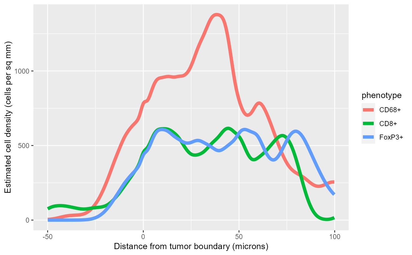
# Plot the densities in a single plot
library(ggplot2)
ggplot(all_rho, aes(X, rho*1000000, color=phenotype)) +
  geom_line(size=2) +
  labs(x='Distance from tumor boundary (microns)',
       y='Estimated cell density (cells per sq mm)')


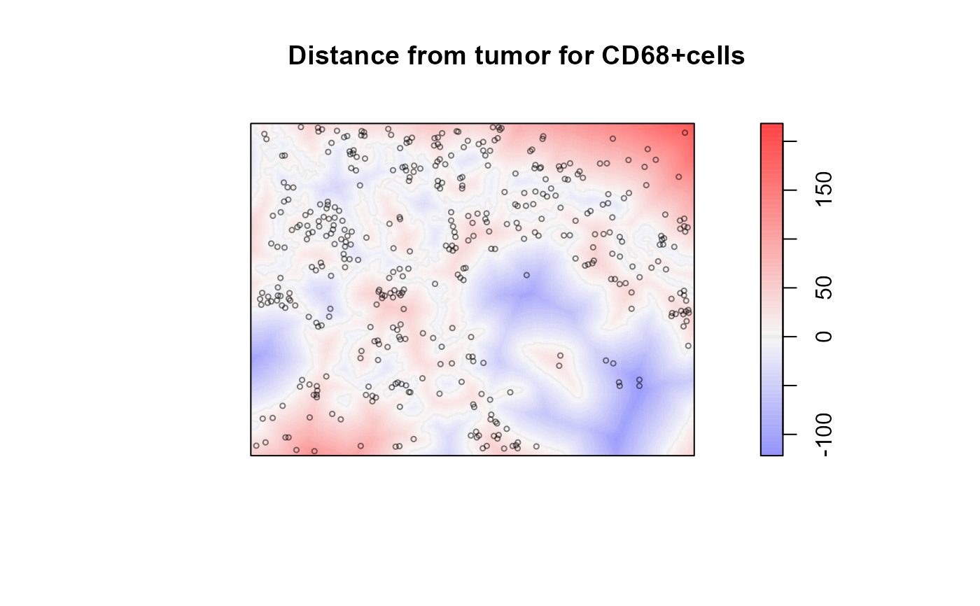
# Show the distance map with CD68+ cells superimposed
plot_diverging(values$distance, show_boundary=TRUE,
  title=paste('Distance from tumor for CD68+cells'),
  sub='Positive (blue) distances are away from tumor')
plot(values$points[values$points$marks=='CD68+', drop=TRUE],
  add=TRUE, use.marks=FALSE, cex=0.5, col=rgb(0,0,0,0.5))